
Understanding the various sources of heating in the atmosphere, like convection and radiation, is critically important in Tropical meteorology. Unfortunately we cannot just go out and directly measure the temperature tendency from convection. However, we can measure the temperature and estimate how it changes as a result of air flowing over an area, and then calculate the “leftover” residual temperature tendency to get an idea of how diabatic processes (i.e. convection and radiation) are heating the atmosphere. In practice, there are two widely used approaches to produce these estimates, and the goal of this article is to provide a brief comparison of them.
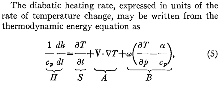
Yanai et al. (1973) were one of the first to explore this idea with data collected from a field campaign. Their approach was to use the dry static energy (DSE),
![]()
which is conserved for an air parcel as long as no diabatic heating occurs. In other words, as long as there is no condensation, evaporation, or radiative cooling, then the DSE value will stays the same, even if the parcel moves vertically and experiences adiabatic heating or cooling.
Using the DSE budget, the net diabatic heating can be diagnosed as follows,

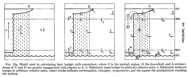
I usually cite Yanai et al. (1973) when doing this calculation, however I recently realized that this idea had been used in earlier studies. One example is Reed and Recker (1971), in which they calculate the heat budget from a triangular sounding array in the West Pacific.
Similar to Yanai’s work, Reed and Recker also parse out the details of convective vs. non-convective regions in terms of their mass, heat, and moisture variations. It’s pretty interesting to compare this paper with the work of others that followed.
Anyway, a slightly different approach is used by other studies such as Nigam (1994), Nigam et al. (2000), and Hagos et al. (2010), use potential temperature (θ), defined as

Potential temperature has the similar conservation properties as DSE. The budget can then be written as,

The ratio in the front simply represents the conversion from θ to absolute temperature, although the units stay the same.
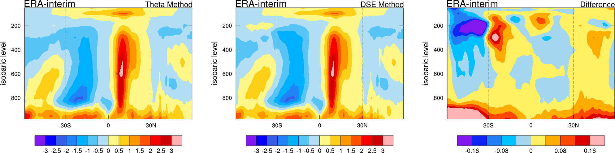
So to compare these two methods I grabbed some 6-hourly ERA-interim data for the month of August 2016, and calculated the heating estimates with both method and averaged them over the entire Tropics (30°S-30°N). Here’s the result:
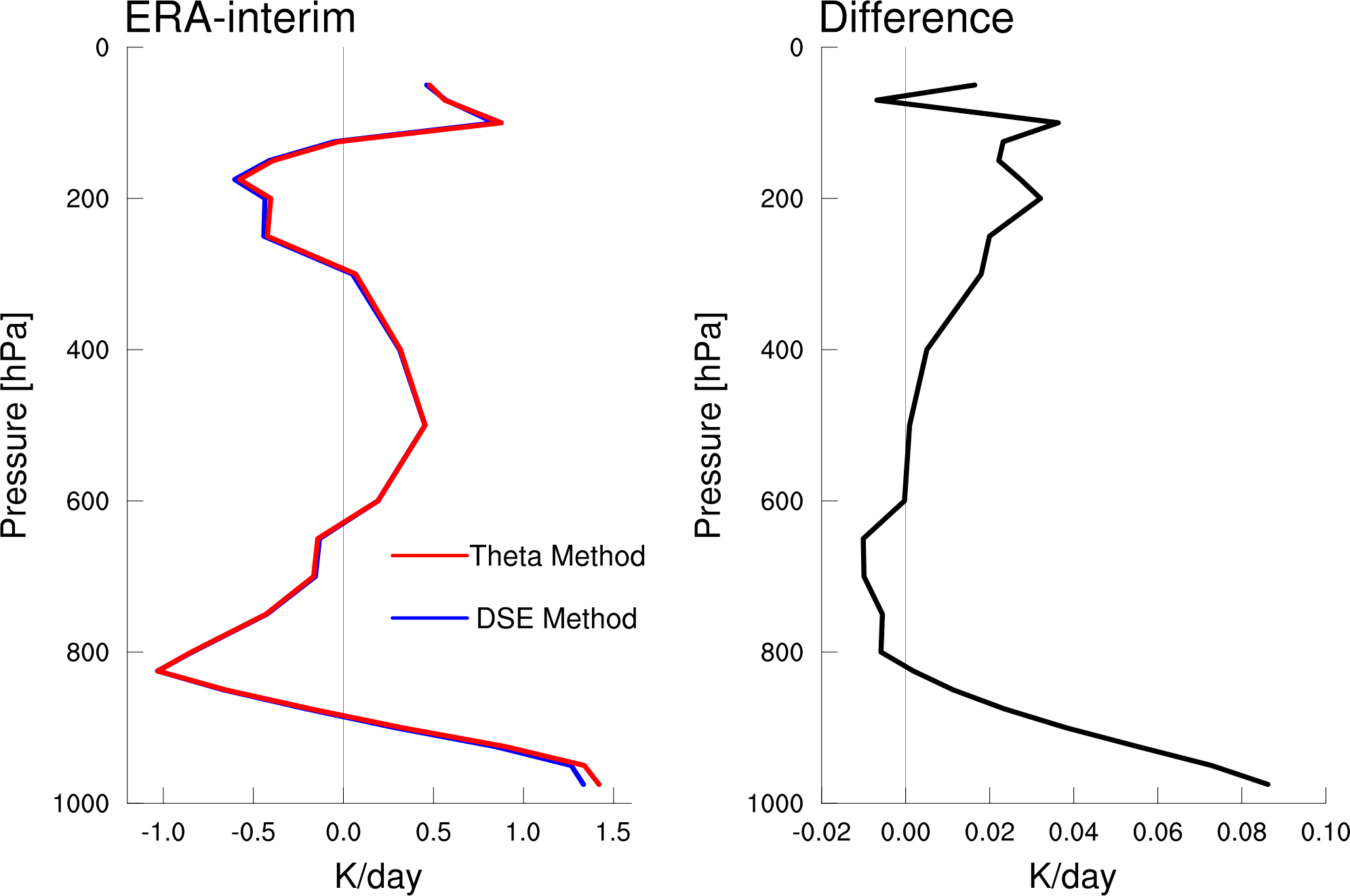
Both methods give a similar average profile with small differences. As Darrell Huff said in his book “How to Lie with Statistics“:
“A difference is a difference only if it makes a difference.”
So is this difference anything to worry about?
The heating near the surface is mostly associated with boundary layer turbulent fluxes that communicate the surface latent and sensible heat fluxes vertically. The heating at the top of the troposphere is partly due to shortwave heating of ozone. The mid-tropospheric heating maximum is mostly due to heating from convection. There is also a small longwave radiative cooling throughout the troposphere, which is overwhelmed by the other processes. In spite of the non-zero heating the Tropics does not continue to get hotter because the general circulation exports a good deal of heat toward the poles.
The difference in the right panel above shows that the method using θ gives slightly more warming on average, which seems really small, but I was surprised that difference was concentrated near the surface and top of the troposphere.
If we look at the differences in just the horizontal and vertical advective components of each equation, the difference of horizontal advection explains most of the difference shown above.
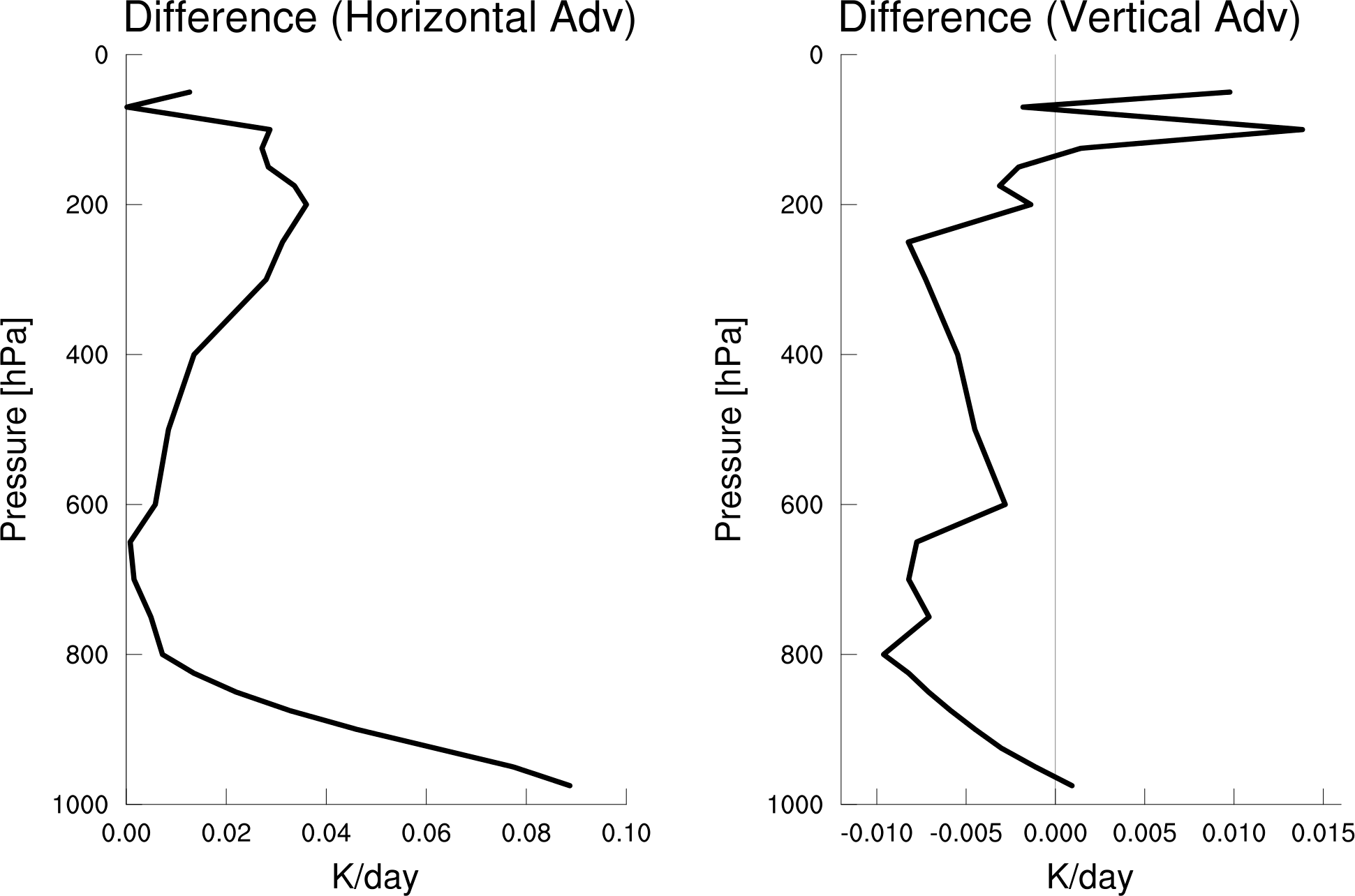
If we do a zonal average we can see these differences are largest away from the equator and away from the regions with the most convective activity, particularly around 25°-30°S.
Although the average difference is small (<0.1 K/day), the difference can be quite large for any given local 6-hourly estimate. This is illustrated by the profiles of the minimum and maximum difference below, as well as the standard deviation of the difference.
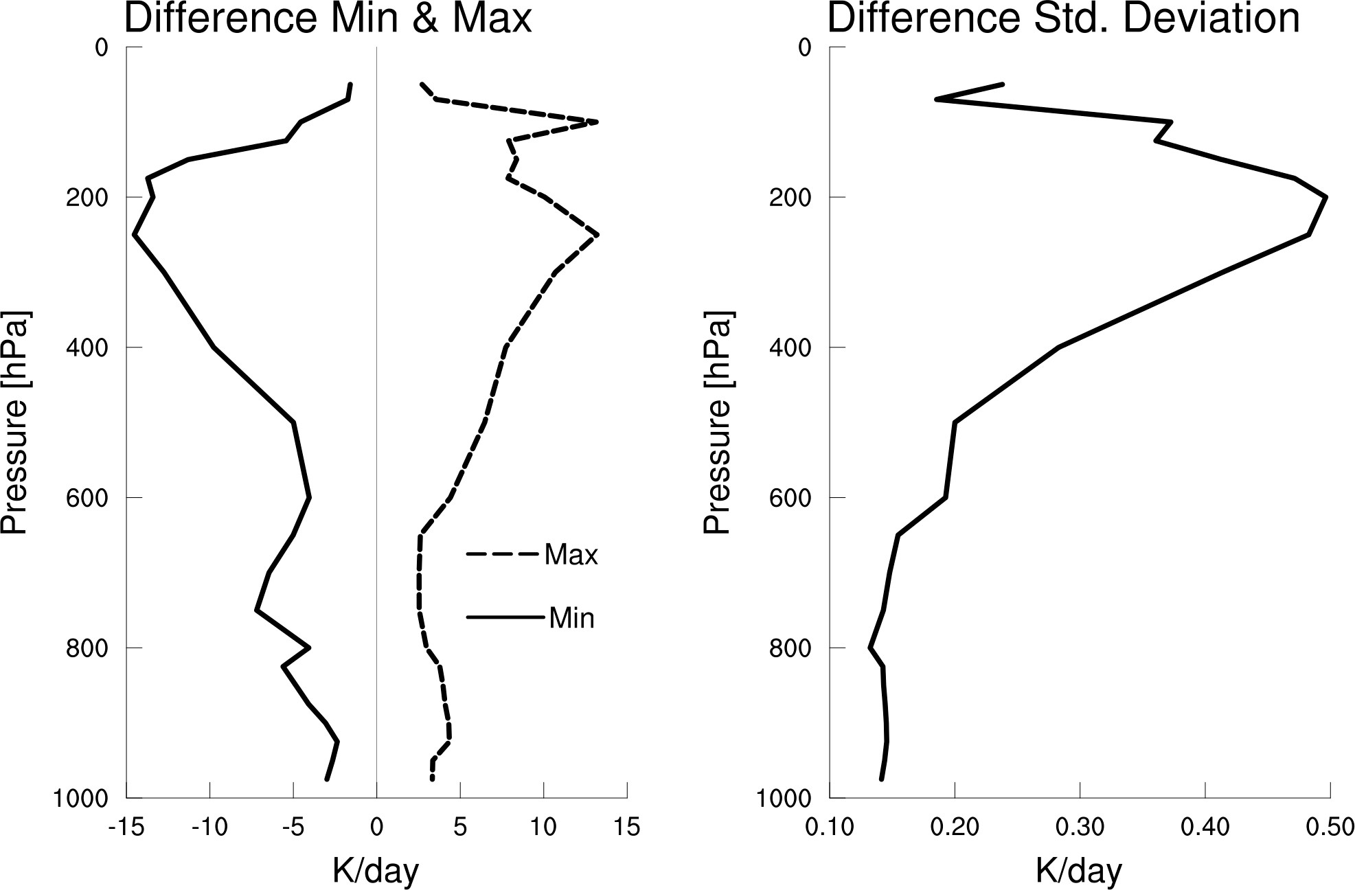
So the differences between the two methods can be quite large at times, and it seems this could make a difference in our interpretation of the data. But why are they different? Or more importantly, which one is more accurate? Ultimately, I’m not sure how to tell.
Part of the answer lies in the linearity of DSE and non-linearity of θ and how this influences the horizontal gradients of DSE and θ. This can be seen by using some basic derivative rules to expand the horizontal advection terms, although it gets messy.
I’m still pondering why these differences exist. I’m inclined to speculate that there may be times when hydrostatic balance is invalid, which could point to the θ method being superior, but I need to think about this more.
Hi Walter,
Thank you for your help and teachings.
Could you please share the NCL script for calculating diabetic heating using these two methods.
Thank you.
Michael, the srcipt is in a bitbucket repository here:
https://bitbucket.org/whannah1/obs-era/src/master/plot.ERAi.Q1_comparison.v1.ncl
It might not be very helpful because it relies on a few other NCL libraries I’ve made. I think it should be viewable without logging in, but let me know if you run into trouble.
The functions for calculating derivatives, like calc_ddx(), can be found in this file:
https://bitbucket.org/whannah1/ncl/src/master/custom_functions.ncl
And the functions for loading ERAi data are here:
https://bitbucket.org/whannah1/ncl/src/master/custom_functions_ERAi.ncl
but the loading functions are somewhat hardwired to the way my ERAi data files are set up. So its probably best to just put in your own code for loading the data.
Thank you so much.
HI, in https://bitbucket.org/whannah1/obs-era/src/master/plot.ERAi.Q1_comparison.v1.ncl
iQ1_DSE_horz = ( U*calc_ddx(S) + V*calc_ddy(S) + W*calc_ddp(S) )*86400.
i am double about why horizontal term includes W*calc_ddp(S) ?
Dear Walter,
Thank you for sharing your codes. They are really usefull.
I don’t understand why it is “S = ( T*cpd + Z )/cpd” rather than “S = ( T*cpd + g * Z )”.
Appreciate if you could give some details.
Thank you.
Im glad you found the code useful! In this case the variable Z already contains the “g” factor, and dividing by cp=1004 just changes the units to Kelvin, which I prefer to J/kg. So it’s essentially the same as the version you mention.
HI, walter!
in your NCL code Q1_comparison.v1.ncl
iQ1_DSE_horz = ( U*calc_ddx(S) + V*calc_ddy(S) + W*calc_ddp(S) )*86400.
i am double about why horizontal term includes W*calc_ddp(S) ?
Ah, good catch! This definitely looks to be a mistake on my part. I don’t have that data lying around, so it’ll take me awhile to fix it. I don’t think the general conclusion will change much though.
EDIT: Actually, after looking more closely at the code, I think the plots are correct. It seems that I went back and changed how that variable was defined to make the plot lower down that shows the min/max and std deviation of the difference. This was pretty sloppy, so I apologize for that. I could have written the code to be much clearer. But if you want to reproduce the plot that shows the difference in horizontal and vertical terms you’ll need to correct that line.
did you use the whole 2016 Aug 6 hourly data or just some of that month? I wanna do some verifications.
Yea, I think I used the whole month.
Hi Dr Walter,
May I ask what range of 6 hourly data in Aug 2016 you used to calculate the above figures? I wrote a Q1 python code based on potential temperature calculation but hope to get some verification.
Thanks!!
Pretty sure I used the whole month of August.
Dr. Walter, could you please tell me how the advection term, which has velocities in meter per sec, is used to calculate the K/day heating rate? I am not able to find it out.
The advection is a velocity multiplied by a gradient. So for a quantity with units of Kelvin, the units of advection are [m/s]*[K/m] = [K/s].
Hello,
I would like to use your code to calculate diabatic heating using theta.
When I load your “custom_functions.ncl”, NCL is looking for other custom functions below:
load “$HOME/NCL/constants.ncl”
load “$HOME/NCL/custom_functions_setres.ncl”
load “$HOME/NCL/custom_functions_qplot.ncl”
I would like to ask where can I find these files.
Thank you in advance for the help.
Hi, those are my own custom libraries of various NCL routines. You can find them here:
https://bitbucket.org/whannah1/ncl/src/master/
But I should warn you that I don’t use NCL anymore, so I haven’t updated anything in several years.
Hello,
When I applied this code. There are no values at 1000 hPa.
Do you have any idea on what is causing this?
That’s due to how I perform the vertical derivative with a centered finite difference. There are ways to avoid this, but I prefer to keep it simple and indicate that those levels contain “missing” data.