A “pointer”, in computer science terms, is an object that references a place in memory. This differs from a variable or an array, because a pointer does not have a type or size that changes. This allows some useful things that are impossible with regular arrays, such as having an array of pointers where each element points to an array of a different size. I recently found a nifty trick in NCL that provide a similar advantage.

Many of my plotting scripts are used to compare different datasets and they generally have this layout:

dataset = (/"Obs","model"/)

do n = 0,dimsizes(dataset)-1
    
    X = < load dataset n >
    Y = < do some calculation >

    if d.eq.0 
        plot = < create XY plot of derived variable Y >
    else
        < overlay XY plot of "model" data to compare with "obs" >
    end if

    delete([/X,Y/])

end do

The main advantage of this approach is that you load each dataset and then clear it when you are done, which saves memory. You don’t have to force them into the same array size wen they have different coordinate arrays.

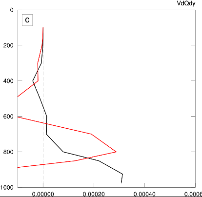
The downside that I constantly run into when making “y vs x” plots is that there’s no easy way to automatically determine the bounds of the plot to ensure that the overlayed data stays within the edges.

An example of the problem can be seen below. Here I plotted the black line first, which set the left boundary so that it would cut off the red line!

The “trick” that I just learned is that you can “attach” arrays of varying sizes to a dummy variable as attributes. Furthermore, you can use the $$ syntax to have the attribute name reflect some incremental variable. Here’s a simple example to explain:

dataset = (/"Obs","model"/)
D = new(1,float)
do n = 0,dimsizes(dataset)-1
    
    X = < load dataset n >
    Y = < do some calculation >

    D@$("Y"+n)$ = Y

end do

Here we have attached the processed variable Y to the dummy variable D as attribute “Y1”. The $()$ syntax allows us to put any string inside the parentheses so we can attach any number of “Yn” attributes.

After this loop we do another small loop to determine what the plot boundaries should be.

pmin := 0.
pmax := 0.
do n = 0,dimsizes(dataset)-1

    tmp = D@$("Y"+n)$

    pmin := min((/pmin,min(tmp)/))
    pmax := max((/pmax,max(tmp)/))

end do

And finally set the resources accordingly:

res@trXMinF = pmin
res@trXMaxF = pmax

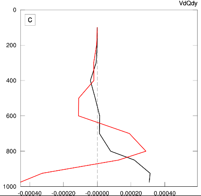
Now we have the desired result where the plot boundaries are determined by all the curves that we need to display, and no data falls outside the edges.

This isn’t what I would call an “elegant” approach, but it might be a useful workaround in a few instances.