I still struggle with using potential vorticity (PV) to think about atmospheric phenomena, but many extremely smart people find it very useful, so it’s a good thing to study. PV is perhaps most often used to discuss circulations on very large scales, but there has been a lot of work to make “PV thinking” work for mesoscale circulations as well. This paper describes such a theory to utilize PV to understand the maintenance of long-lived mesoscale systems in which convection plays a substantial role.
Self-maintaining mesoscale phenomena such as supercells and squall lines are often described in term of processes that act on the “fast manifold“, which means that the Earth’s rotation does not play a role (i.e. Rossby number is larger than one). On the other hand, slow manifold dynamics can be simplified with the geostrophic approximation, in which the Coriolis torque is relatively large (i.e. Rossby number is small).
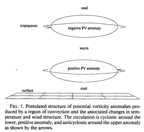
The main hypothesis of the paper is illustrated in Figure 1 (below) and the way in which convection is assumed to affect the vertical distribution of potential vorticity.
“Since the primary action of cumulus convection is to transport mass across isentropic surfaces, the effect of cumulus convection on the potential vorticity distribution is easily understood. If the mass-integrated potential vorticity remains constant between two isentropic surfaces, then evacuation of mass from this layer will decrease the mass and increase the potential vorticity.“
Another way to think of this is that convection is moving mass “upward” across isentropes while also moving PV “downward“. To be honest, I have a hard time thinking about this.
The effects of evaporation, melting, and radiation can cause PV to be moved around, but the details can be very complicated depending on how the convective anvils form. For example, a convective anvil top radiatively cools and fluxes PV upward, while the anvil bottom radiatively warms and fluxes PV downward. Thus the radiative impact of PV is highly sensitive to the thickness and size of the anvil. The authors mention that field study estimates suggest radiative impacts below the anvil can be as large as 2.0 PVU/day, which is large considering mid-tropospheric PV is typically around 0.6 PVU. In any case, all three of these convective processes generally increase lower tropospheric PV, so they do not change the qualitative picture in Figure 1.
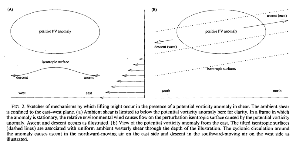
Assuming that the isentropic surfaces are not distorted very fast by the ambient shear, the vertical motion can be understood in terms of how the air flows up and down the isentropic surfaces. For the scenario in Firgure 1, the ways in which vertical motion can occur can be described as a combination of two processes:
- The ambient circulation will cause air to flow underneath the PV anomaly, forcing air to ascend as it approaches the anomaly and descend as it exits (Fig. 2a).
- Assuming westerly shear, the circulation of the anomaly will force the air to ascend on the east side (ie.e downshear) of the anomaly, and descend on the west side (Fig. 2b).
One thing that confuses me about Raymond and Jiang’s description here is how the shear is important. It seems this whole picture would be the same in an unsheared environment. Maybe I’m missing something….
[EDIT]
I realized why this is important! I forgot that the shear is “storm relative”. Without a sheared profile there would be no storm relative inflow at low levels. We could assume that the storm is moving with the larger scale flow, thus the mechanism in Fig. 2A would not work.
[/EDIT]
In any case, the main questions are,
- Can convection create a PV anomaly strong enough to induce lifting of boundary layer air?
- Will the ambient shear “that makes this lifting possible” allow the PV anomaly to survive long enough for the mechanism to act?
Non-Linear Balance
The model uses a “non-linear balance” approximation, which is described in much more detail by Lorenz (1960) and McWilliams (1985). I had never heard of this approximation before so I did some further digging. Raymond and Jiang describe this simply as,
“The nonlinear balance condition arises from replacing u and v in the horizontal momentum equation by -∂ψ/∂y and ∂ψ/∂x, and further assuming that the vertical velocity is negligible.”
Another explanation can be found in an older paper, Raymond (1992), in which Raymond puts non-linear balance into a more thorough historical context. From Hoskins et al. (1985), the invertibility of potential vorticity relies on a balance condition that is approximately satisfied by the flow.
There are many valid choices for this balance condition depending on the scales of interest. For instance, geostrophic balance is approximately valid for small Rossby numbers (i.e. Coriolis torque is relatively large), but is not valid for mesoscale circulations like supercells and squall lines. There is no fundamental limit on invertibility, it can work on any scale, but finding the “right” balance condition becomes the central problem. Raymond (1992) then describes how non-linear balance fills this role for mesoscale phenomena.
“Nonlinear balance is a possible candidate for a balance condition on short timescales.
It is approximately valid when circulations are nearly horizontal, and it is obtained (in most cases) by dropping all terms in the divergence equation containing the divergence, the vertical velocity, and the divergent components of horizontal velocity. Bolin (1955, 1956) and Charney (1955, 1962) were the first to use nonlinear balance in numerical models. However, Lorenz (1960) was the first to develop a nonlinear balance approxi- mation to the primitive equations in a manner that conserved an energy-like quantity. In the Lorenz model all first-order terms in the vorticity equation involving the divergent part of the wind must be retained. The Lorenz model thus arises from an inconsistent truncation of the primitive equations, since only the leading-order terms are retained in the divergence equation.”
Raymond (1992) also nicely illustrates that non-linear balance can be obtained in several different ways,
“In the Lorenz model only a single prognostic equation survives. Both the vorticity equation and the thermodynamic equation retain time derivatives, but the nonlinear balance equation relates these, making one into a diagnostic equation for the vertical velocity. The vorticity equation is generally taken to be the prognostic equation.
Charney (1962) used a different approach to integrate the nonlinear balance equations by taking the potential-vorticity equation rather than the vorticity equation as the prognostic equation. The diagnostic equation relating the pressure or stream-function to the potential vorticity is more complex than the equivalent relationship for the vorticity, which makes the mathematical solution more complex. However, the potential vorticity approach has the attractive feature of making the mathematical procedure congruent with the conceptual picture of the inversion process.”
Thoughts on the Model Derivation
I don’t fully understand the model derivation. For instance, the authors define the streamfunction and velocity potential,
![]()
![]()
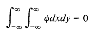
and then mention this caveat,
“Given u and v, the determination of ψ and φ is not unique because there exists a flow component that is both irrotational and solenoidal that can be assigned to either ψ or φ. However, we insist that
… then the ambiguous part is uniquely assigned to ψ.”
At first I thought this similar to requiring the flow be non-divergent, but that’s definitely not the case. So… what does this mean? How does it affect the potential vorticity?
Another simplification that confuses me,
“The term (∂b’/∂z)∇ 2ψ has been dropped even though it is formally of the same order as the other non-linear terms. This is consistent with the later approximations in which the perturbation vertical gradients are ignored compared to the ambient vertical gradients in vertical advection terms.”
This seems weird because the vertical gradients of perturbations seeem to be important. Maybe the idea is to ignore perturbations on what might effectively be called the “cloud scale”, which buoyancy and drag are the dominant forces?
I’ve never built or run a model like this, so I was a bit surprised about some of the details. For instance, the domain is periodic in the east-west direction, but geostrophic balance is enforced at the north and south walls of the domain. One reason for this might be a way to insure that PV cannot be created or destroyed, except at the surface, since this would ensure no “convective activity” at the boundaries.
Also, the grid seems surprisingly small and coarse at 17x17x17 with a 100km grid spacing.
Results
So back to the main questions! The authors want to know if the PV anomalies created by convection can foster more convection, and become self-sustaining. To answer this they initialize the model with a PV anomaly and run it for 24 hours. The resulting picture in Figure 6 shows upward motion to the east and descending motion to the west.
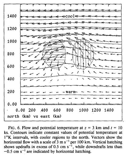
The upward vertical velocity anomalies are on the order of 1 cm/s, which allows parcels to ascend up to 500 m. They argue that this is sufficient to “release conditional instability”, or in other words this can initiate convection. This is summarized in the last section as,
“We postulate the existence of self-maintaining mesoscale convective systems based on an interaction between convection and slow manifold dynamics.”
Seems like a lot of work just to make that statement!
They note one small, but important caveat about the magnitude vertical motions in large balanced vortices compared to those in organized convective systems,
“Perhaps the weakest assumption in the present theory is that the tiny, but persistent quasi-balanced upward motions are more important in the long term than the much larger, but transient motions due to fast manifold dynamics.”