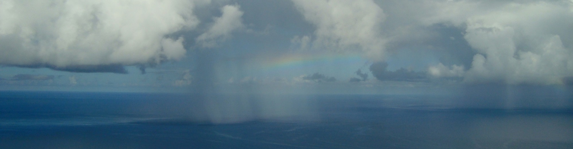
A lot of interesting weather phenomena are associated with various types of atmospheric waves. In most cases, we have a good understanding of wave dynamics when the atmosphere is dry and there’s no condensation or evaporation, but we lack a solid understanding of how things change when moist convection gets involved (i.e. clouds). A good example is how convectively coupled Kelvin waves move at a fraction of the speed compared to their dry counter parts (Kiladis 2009). I recently read the paper below by Paul O’Gorman that discusses a simple way to modify dry theory such that the effects of heating by convection can be implicitly included.
In general, waves move faster when the static stability is higher. I like to think about this in terms of what happens to a vertical displacement. For higher stability, there’s a stronger restoring force on any vertical displacement of air (assuming no latent heating occurs), which speeds up the motion associated with the wave causing the wave to propagate faster (i.e. faster phase speed). Similarly, when the stability is lower, the wave motions will be deeper, and the phase speed should slow down.
When we consider waves with embedded moist convection, we expect clouds to occur in areas where air is going up, but not where air is going down. The tendency for clouds to form where air is going up creates an asymmetry of diabatic heating in a wave (see figure below). When clouds form, the diabatic heating from condensed water vapor warms the air. So the whole rising air mass experiences less cooling than it would in a dry atmosphere. This is similar to what would happen to dry air if the static stability was lower. The basic idea of effective static stability is to estimate this hypothetical stability instead of considering all the complicated things that happen when clouds are present and interacting with the waves.
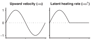
Taken from Fig. 1 in O’Gorman (2011). Idealized horizontal profiles of vertical velocity (left) and diabatic heating (right) to illustrate how convective heating is asymmetric in an atmospheric wave.
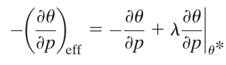
The derivation of effective static stability is pretty straightforward. Dr. O’Gorman provides a nice summary on his website, along with a MATLAB script with a function for calculating individual profiles of the effective static stability. A key point of the derivation is to obtain the Eulerian tendency of perturbation potential temperature (θ’).
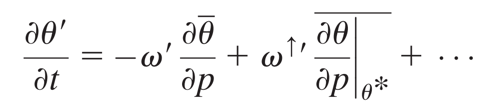
The equation also includes terms from other stuff (radiation, advection, etc.), but we don’t need to worry about these for now. The first term on the right hand side represents the θ change due to dry vertical motion (i.e. no clouds). The second term represents the θ change due to convective heating, which only occurs when vertical motion is upward (ω↑‘ is set to zero otherwise). This “saturated ascent” term is written assuming that cloudy parcels are conserving their saturation equivalent potential temperature (θ*), which is an ok assumption here, but technically not true for individual clouds (due to entrainment).
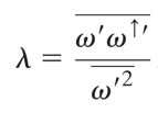
“The central approximation of the derivation is to relate the eddy latent heating rate (or more precisely ω↑‘) to the eddy vertical velocity”
![]()
The rescaling or “eddy asymmetry” parameter, λ, represents the degree of asymmetry between the vertical motion in regions with and without clouds. The last term, ε, represents the error in this approximation.
As a rough global average λ=0.6 is a fair approximation. Dr. O’Gorman doesn’t really talk about the sensitivity of these calculations in his paper. I was a bit curious how much this varied so for my initial attempt to calculate this I defined perturbations relative to the time mean for each month. This allowed me to get an idea of the seasonal cycle of eddy asymmetry and,surprisingly, the monthly λ values had a monthly standard deviation (see below) of up to ~0.1 in the sub-Tropics! I was expecting much less variability, but it seems that this is simply a reflection of how much precip varies seasonally in monsoon regions.
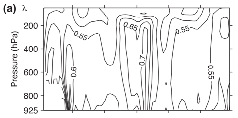
Here is Dr. O’Gorman’s plot of zonal mean λ,
For comparison, here are the values I calculated for λ in the tropics along with the monthly standard deviation,
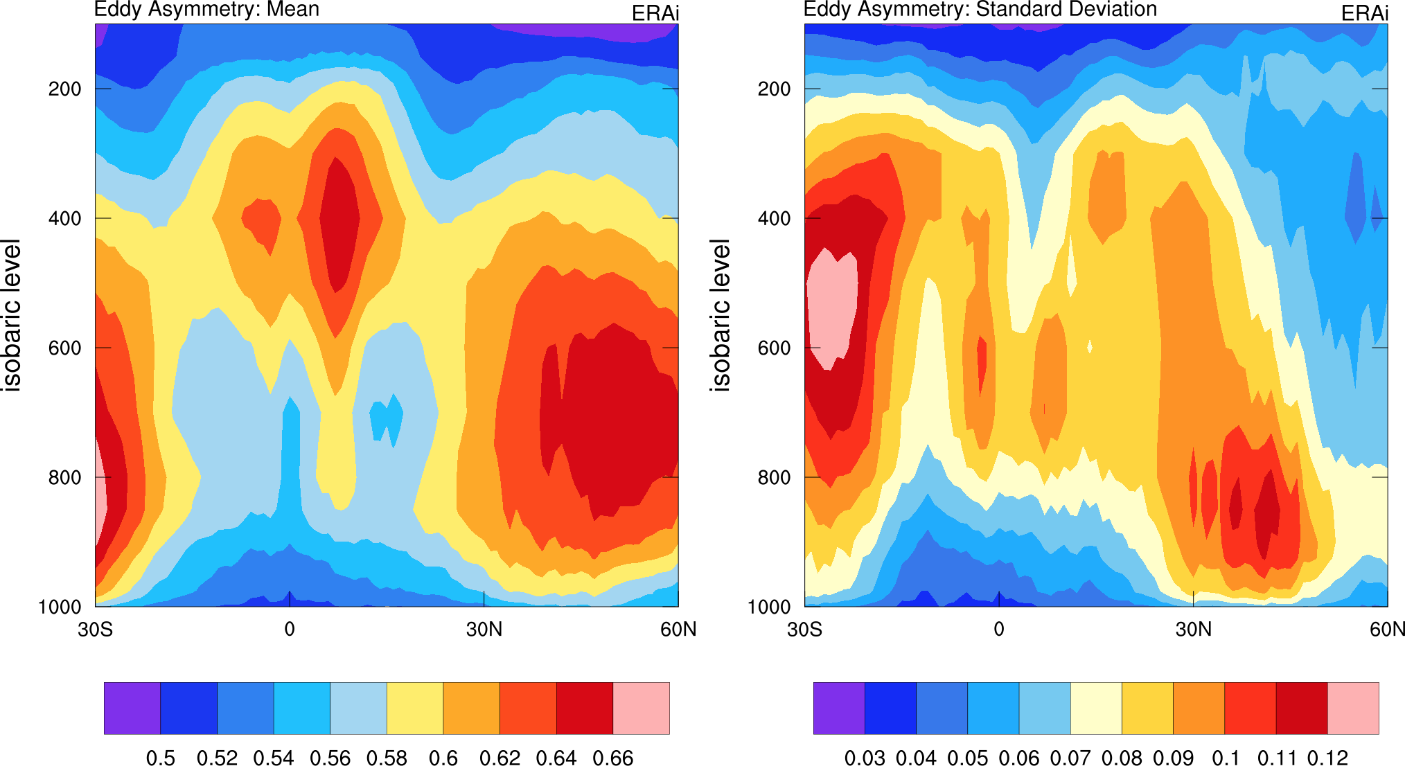
Mean (left) and monthly standard deviation of the Eddy Asymmetry Parameter (λ) calculated from 4x daily ERA-interim data.
The first equation can then be rewritten as,
![]()
where the effective static stability is defined as,
or similarly in height coordinates,
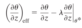
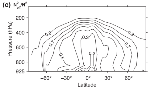
Figure 4c offers a nice way to see how the effective static stability differs from the dry static stability (see below). This shows how the effective static stability is 10-30% of the dry static stability on the equator!
The other sections of this paper about applications of effective static stability are interesting, but I didn’t fully understand the parts about supercriticality constraints (see Schneider and Walker 2006), so I’m not gonna cover those. Nonetheless, the arguments for the use of this theory to understand the more subtle aspects of global warming were very convincing.
I contacted Dr. Gorman about how to calculate λ, and he said that he used a mean over all times and longitudes to define the perturbations. This makes me wonder whether using a long-term average really makes sense for all wave types. The variability that I found could also be a consequence of eddy asymmetry not being the same for all eddies, like stronger or larger eddies being more or less asymmetric. This might be an interesting thing to look further into for a future project.
There’s an interesting note about λ at the end of the paper,
“It remains to be seen if λ remains constant as the climate changes in comprehensive GCMs or in nature. There is a slight increase in λ when the spatial resolution is doubled in the reference simulation of the idealized GCM, but several other circulation statistics also change…”
I think this could be due to a simple change in eddy activity. It’s possible that certain region of a model will have more convectively coupled disturbances as the grid spacing decreases. For instance, the seasonal shift of a monsoon could lead to changes in λ even though the disturbances are not fundamentally different.