Super-parameterization is a type of multi-model framework (MMF), which is a technique for modeling a physical system with a wide range of important scales (such as the climate system). A model is typically designed to simulate things on a certain scale of interest, but it also needs information about things happening on smaller and larger scales. This missing information is condensed into model parameters, which can be fixed or variable. A parameterization* is a method for estimating parameter values without explicitly simulating the processes directly. Parameterizations can sometimes be thought of as very low order models. Super-parameterization replaces one or more parameterizations with a second model that is designed to simulate the processes explicitly, in order to provide more accurate parameter values back to the main “host” model.
* Note that the term “parameterization” used here is different from the mathematical term for parameterization of a function, which is a mapping between a multi-dimensional object and a one dimensional parameter.
My only experience with super-parameterization is in the context of modeling the atmosphere, but it can be applied to other subjects. As a simple illustrative example, consider the typical Lotka-Volterra example of a ecosystem consisting of a population of rabbits (R) and foxes (F).

A model of the system can be written,
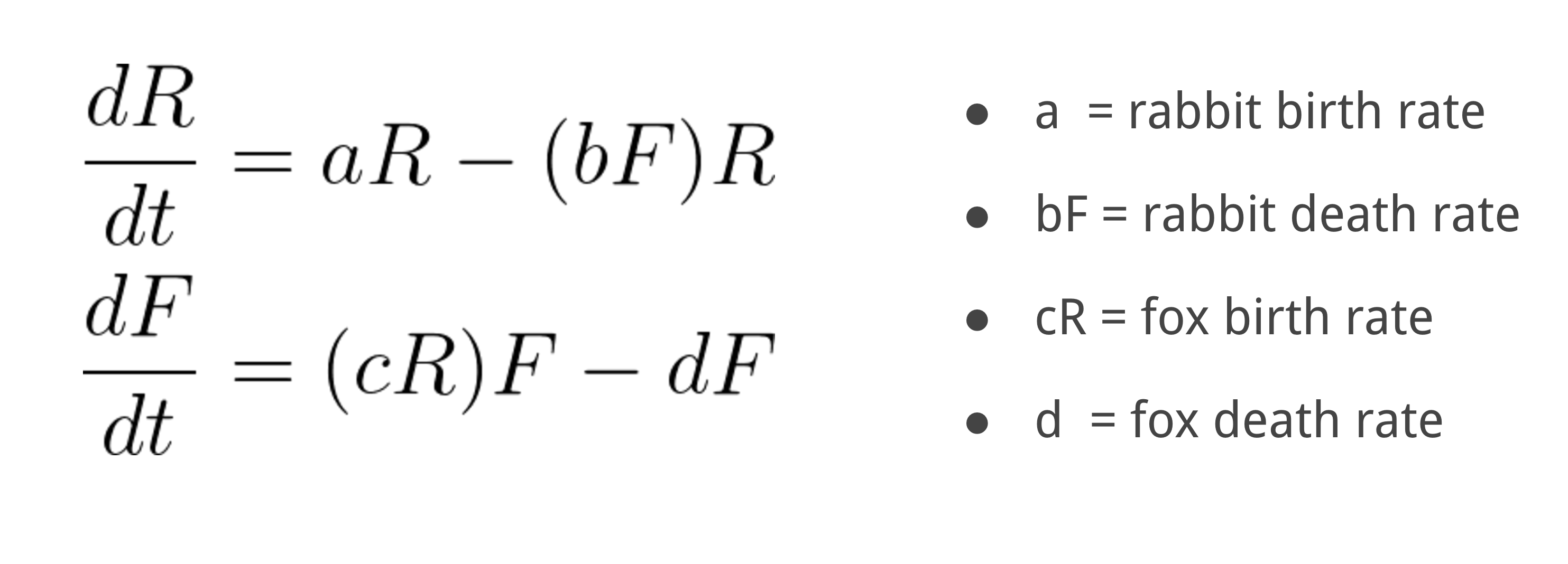
We have 4 parameters (a,b,c,d), and typically we would just assume constant values to explore the population dynamics. Alternatively, we could parameterize these values to represent other processes that are not in the basic model. For instance, maybe foxes are more efficient or successful hunters during summer. This would be simple to parameterize by making the parameter b fluctuate with the day of the year.
Now what if we consider that foxes also become less efficient hunters as they age? This is difficult to parameterize if we don’t assume something about the age distribution of foxes. The MMF approach to this problem would be to use a secondary model that explicitly simulates the lifecycle and hunting efficiency of a small representative sample of foxes in the ecosystem. This would allow the age distribution of foxes to evolve with time, which could then be used to obtain an evolving estimate of the parameter b. Additionally, the fox model could be designed to affect the fox birth rate c, since only mature foxes can reproduce. This would be a “super-parameterization”.
Super-Parameterization in Atmospheric Models
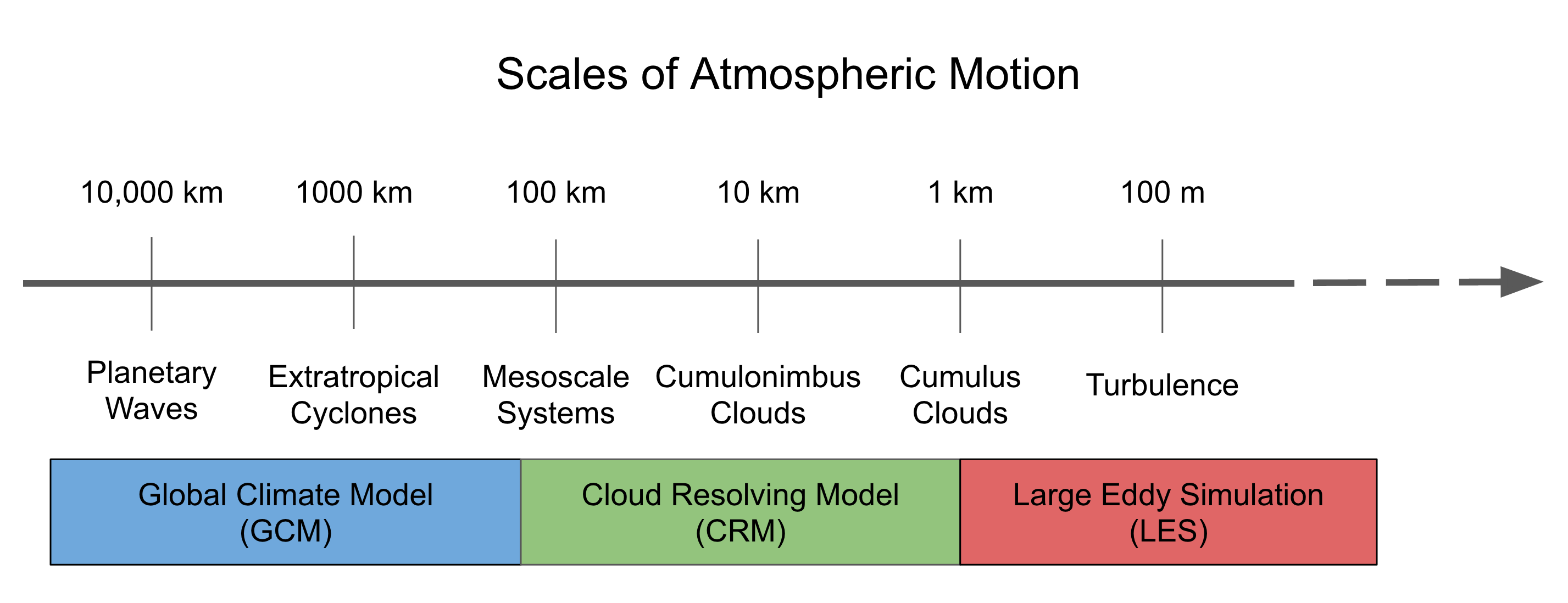
In the context of atmospheric models, clouds are one of the most difficult things to represent realistically when the model needs to cover the entire planet. At the core of this problem is the wide range of important scales in the atmosphere that need to be considered when building a model to simulate the climate system or weather events.
Current parameterization schemes have had mixed results trying to fill the gaps in this spectrum of scales. Sometimes parameterized clouds rain too often and other times they don’t rain enough. Certain types of “organized” storms, like supercells, may not be represented in a model at all. There as also other “small” things, like dust or soot, that affect and are affected by clouds, but these processes are often not treated realistically. Akio Arakawa said it best when he said,
“Cloud parameterization is a very young subject.”
For a good review of the current issues with cloud parameterization check out this paper:
Given that cloud parameterizations are so problematic, they stand to benefit from super-parameterization. Luckily, in addition to large-scale atmospheric models, cloud-scale models have been used for decades to explicitly simulate convection and turbulence, so we have a lot of experience with this. Sometimes these are called “cloud resolving models” (CRM) or “cloud system resolving models” (CSRM). If the model is configured to simulate small clouds or turbulence with a grid spacings of 100 m or less we usually refer to this as a “large eddy simulation” (LES).
One of the first CRM studies was done by Masanori Yamasaki.
More sophisticated models are used these days. The image below was created from a simulation known as the Giga-LES, that used a 1024x1024x256 grid with 100m grid spacing (i.e. a very fine grid over a very large area). The visualization was created with a 3D radiative transfer algorithm (see SHDOM). The Giga-LES was run on a massive super computer and took a long time to finish, but the resulting convection behaves in a realistic manner. In this simulation many different sizes and types of clouds can interact, just like they do in the real atmosphere.

Visualization of the Giga-LES simulation by Ian Glenn. Created with SHDOM.
Couldn’t we use an LES model to cover the whole globe?! Yes…, but, unfortunately, that is too expensive with the computers we have now. However, we can compromise. Instead of a 3D model with a fine mesh, we can use a 2D model with a coarse mesh as a super-parameterization and still do better than a conventional cloud parameterization! The figure below illustrates how this looks.
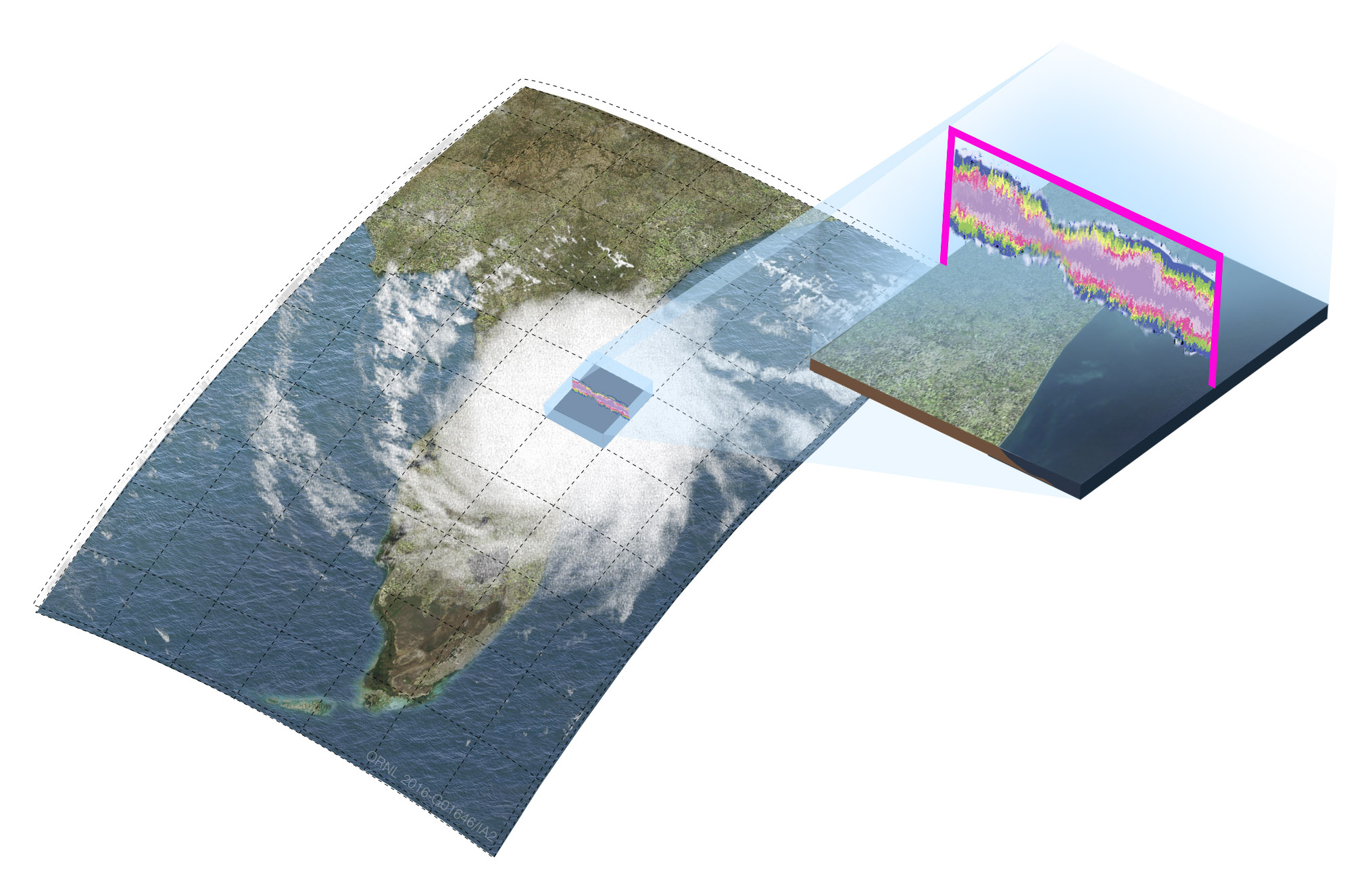
The embedded 2D cloud model takes information about how temperature and water vapor are changing in the “parent” or “host” global model, and explicitly simulates how the clouds will respond. Once the cloud model has run for the length of the host model time step, it passes the resulting information back to the host model, just like a conventional parameterization. This information includes how much rain hits the surface, as well as how the clouds move heat and water vapor around in the atmospheric column.
We get many other benefits from the embedded cloud model. In addition to replacing the cloud parameterizations, the embedded 2D cloud model also calculates:
- radiative heating
- turbulent mixing
- microphysical processes
- gravity wave effects
And since these processes are simulated on the same grid as the clouds, they can interact with each other in a natural way.
Outstanding Issues
In spite of all the promising aspects of super-parameterization, there are some caveats. The biggest trouble with a super-parameterized weather forecast or climate model is that it is still very expensive compared to conventional models. Producing multiple 100 year simulations is currently out of reach, but by utilizing GPU architecture we may be able to overcome this.
Also, the clouds in a 2D model are not as realistic as those in a 3D model. The divergence of air at the top of a 2D cloud cannot spread out in all directions, which affects the dynamics of the clouds. Additionally, 3D clouds have the benefit of being able to accurately transport momentum, although there is a way of treating momentum as a passive tracer in a 2D model. 2D clouds are also limited in the types of storms they can mimic. On the other hand, using a 3D model with a comparable domain size is hugely expensive, so a 3D super-parameterization is usually limited to a small domain that can cause other issues.
There are many other ways we can further improve on super-parameterization. For instance, the embedded CRM does not “feel”any subgrid topography, which can provide lift and trigger convection that is important on regional scales. The CRM also does not know about the diversity of warm and cold spots on the land surface below, or surface heterogeneity, that can affect how clouds form. At some point it may be interesting to include vegetation in a super-parameterization to see how evapotranspiration might change when explicitly coupled to convection.
More Info
For more about the current state of cloud parameterization and super-parameterization, check out these articles:
Randall, D. A., 2013: Beyond deadlock, Geophys. Res. Lett., 40, 5970–5976.
Can I translate it to Chinese and share it in my Wechat?
Sure, just cite the source with a link.
I would add that SP also often acts as a “notch filter”, excluding the mesoscale (~100km scales of motion) or in other words it enforces the old hypothesis of scale separation. This is just a mathematical truth: there are no fluid motions in SP models on scales between the span of the cloud model and the mesh spacing of the large-scale host model. Even if those ranges overlap, it prevents scale interactions (communications between scales) of the sort envisioned in many “multiscale” views of fluid flow, like the turbulent cascade.
SP embodies the null hypothesis about mesoscale motions: that they don’t matter. In this light, I find especially interesting the successes (and the question of whether our diagnoses can detect systematic shortcomings of) very-small-CRM SP models, like in
Pritchard, M. S., C. S. Bretherton, and C. A. DeMott (2014), Restricting 32–128 km horizontal scales hardly affects the MJO in the Superparameterized Community Atmosphere Model v.3.0 but the number of cloud-resolving grid columns constrains vertical mixing. J. Adv. Model. Earth Syst., 6, 723–739, doi:10.1002/2014MS000340.
Parishani, H., M. S. Pritchard, C. S. Bretherton, M. C. Wyant, and M. Khairoutdinov (2017), Toward low-cloud-permitting cloud superparameterization with explicit boundary layer turbulence, J. Adv. Model. Earth Syst., 9, doi:10.1002/2017MS000968.
Excellent point!
Thanks Walter for a well articulated summary of SP.